The Relative Strength Index is a popular indicator for developing short-term long-only strategies but careful analysis shows that its performance depends on price action dynamics and as a result ex-ante parameter selection is hard or impossible.
In my book Fooled By Technical Analysis I outline a procedure for testing trading strategies for robustness for the purpose of determining whether they are random. The two-day Relative Strength Index (RSI2) is one of the strategies I show to be random and an artifact of data-mining.
But what do we mean when we say that a trading strategy is random?
Although we could probably come up with several fancy definitions of what a random trading strategy is in the context of statistical analysis, a practical one is as follows:
A trading strategy is random if it requires special market conditions to perform well and when these conditions are not present its performance deteriorates.
In other words, a random strategy does not exploit atemporal structural anomalies in price action but temporal anomalies that appear and disappear as market conditions change. For example, the cross-sectional momentum anomaly has been shown to be structural so far while the time-series momentum anomaly comes and goes depending on market conditions.
Back to RSI2: Why is this strategy random?
We will show that the RSI2 strategy exploits temporal anomalies and its performance depends on the value of the parameters used, which cannot be determined ex-ante.
Although there are many variations of the strategy, we will deal here with its popular core, which is as follows:
Buy if RSI(2) < OS
Sell if RSI(2) > OB
OB and OS are the oversold and overbought levels.
Note that adding more rules, as it is done usually, for example moving average cross conditions, etc., only increases the data-mining and data-snooping biases. Here we would like to determine whether the basic idea works. If it does not, adding more rules to force it to work causes data-snooping bias.
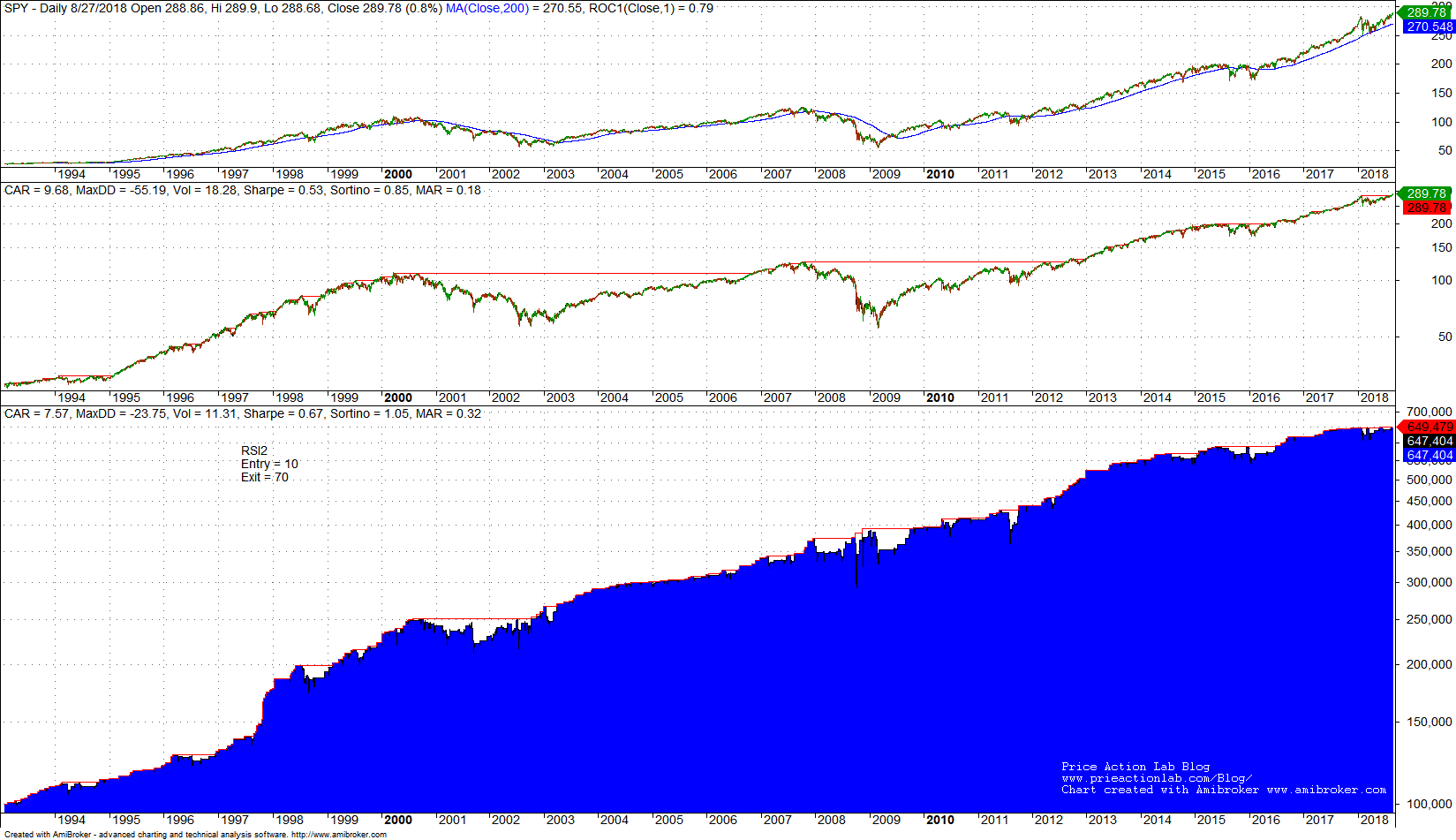
Below is the performance of this strategy for OS = 10 and OB = 70 in SPY ETF from inception on 01/29/1993 to 08/27/2018. Commission of $0.01/share is included.
Although CAGR for the strategy is 7.57% versus 9.68% for buy and hold (shown in middle chart), risk-adjusted performance is higher with MAR (CAGR/Max. DD) for the strategy at 0.32 versus 0.18 for buy and hold. This looks good, but wait!
How did we come up with those values for the parameters OB and OS? Obviously through trial-and-error or optimization, both of which can lead to multiple comparisons and eventually to data-mining bias.
Note that the strategy with the above parameters has had only one down year in 2001 with -5.2% return. Even 2008 is positive with +3.7%. But year-to-date the strategy performance is at 0%.
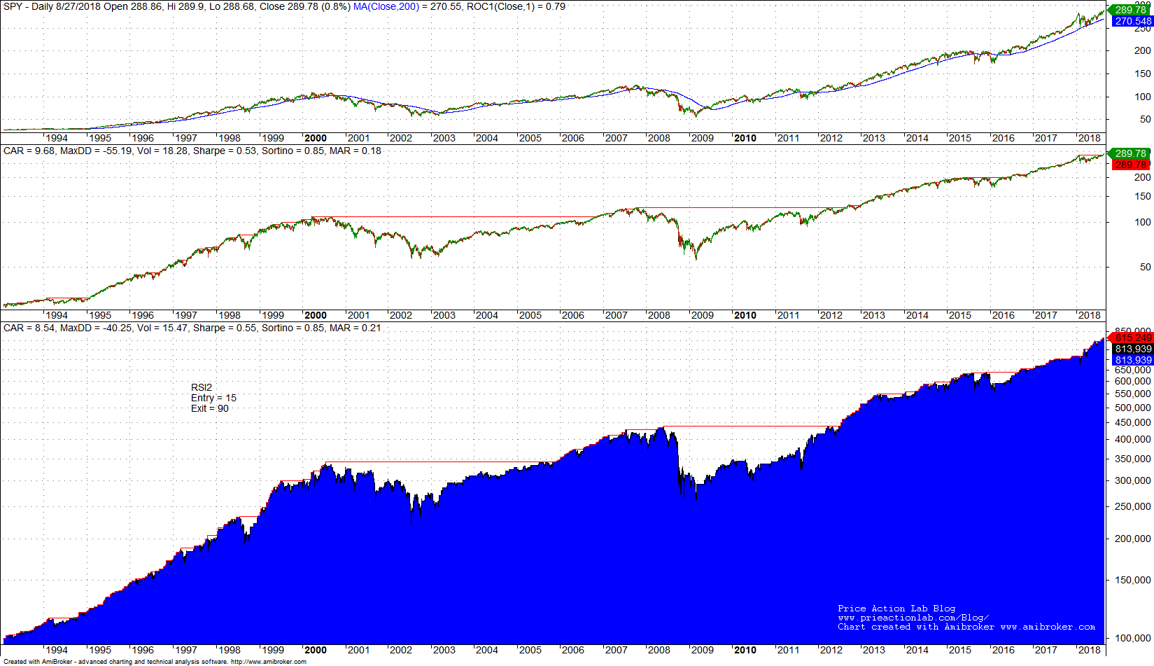
Maybe we could increase CAGR for the strategy and year-to-date performance by setting OB = 15 and OS = 90. Below is the equity performance.
In this case CAGR is 8.54%, higher by 1% but maximum drawdown increases to -40.55% from -23.75%. As a result, MAR falls to 0.21, close to buy-and-hold performance and performance appears random.
Let us try to understand what happened here: OS = 95 delays the signal exit and allows capturing more profit. As a result CAGR increases but that comes at the expense of higher drawdown when market conditions are not favorable. Despite the higher CAGR, there are now four losing years with 2008 at -24%! This means that the parameters selected optimize performance during favorable conditions but when conditions are not as favorable, performance deteriorates. This is the result of over-optimizing on favorable conditions. Note that with the new parameter values, year-to-date return is +13.2% versus 0% with the previous settings. This is a huge variation than points to random behavior.
Therefore, the performance of this strategy depends on some favorable conditions and selecting the right parameters. Obviously, no one knows market conditions in advance and cannot select the best parameters. Due to this, some traders that use this strategy to trade or sell signals with the wrong parameters have underperformed SPY buy and hold year-to-date and are wondering what happened. Actually, what happened is that market conditions changed.
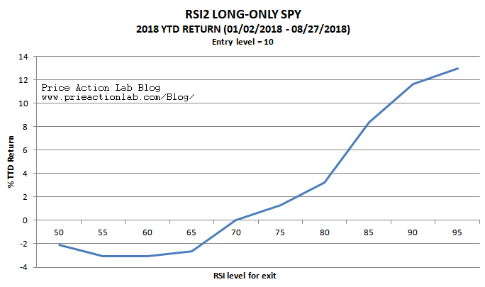
Let us look at some graphs for 2018 only. A 3-D graph would be best but could be difficult to interpret so we will stay with 2-D graphs and start with setting OS = 10 and varying OB from 50 to 95, as shown below.
It may be seen that profitability year-to-date is negative for OS < 70 but then becomes positive and increases as OB increases. Actually, any random buy-the-dip entry signal could have same performance as the RSI2 provided that the exit signal maximizes profit. In other words, the exit signal is important, not the entry.
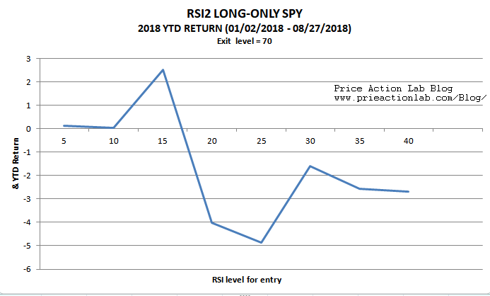
In the graph below we set OB = 70 and vary the OS entry level from 5 to 40. It may be seen that performance is flat or negative except for OS=15.
We could go on forever showing graphs but the reader probably gets the idea: the RSI2 is fundamentally a buy-the-dip strategy and profitability depends on capturing profit after a bounce. Usually, during strong uptrends, such as the one this year, the profit is higher after a bounce and this is why OB=95 seems to work better while the entry level OS is almost irrelevant and any strategy that buys dips could do as well.
But in bear markets, rebounds do not last long and timing of exits matters more. This is why exiting as fast as possible works well and OB = 70 results in flat performance in 2008 while OB=95 generates a large loss. These effects can also be seen from the two equity charts above.
Conclusion
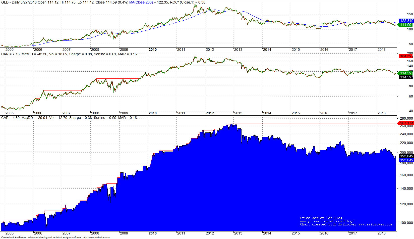
So is the RSI2 a random strategy? The answer depends on the criteria for randomness and according to the ones in this article it is a random strategy. Actually we have developed a variety of similar strategies that do not use the RSI2 but other indicators that behave in similar ways and results are similar. These strategies buy dips but performance does not depend so much on the entry but on the exit. Specifically, for OS=10, OB=70, RSI2 return for 2008 was +3.7%. But keeping OS=10 and changing OB to 90, results in -21.2% loss for the same year. These variations are huge and strong indication that the strategy does not exploit a structural anomaly but specific market conditions that usually change. For example, year-to-date, OB=10, OB=70 performance is flat but OB=10, OB=90 yields +11.6%, above buy-and-hold. There is no way of knowing what parameters to use in advance as market conditions change randomly and do not issue warnings. Trading strategy developers can follow certain procedures such as the one outlined in the book Fooled By Technical Analysis when trying to determine whether a strategy is random. For example, below is the performance of RSI2 with OS=10, OB=90, in GLD since inception.
The strategy worked well in the GLD uptrend but failed consistently in the downtrend. One reason is that market conditions changed after the uptrend and rebounds did not last as long. Actually, the strategy has negative performance for all combinations of values for OS from 5 to 40 and for OB from 50 to 95 after 2014 although it worked well before during the uptrend.
Adding more filters and parameters after knowing initial results increases data-snooping bias and the forward results are random with high probability, as this article shows. If the core of an idea points to randomness, adding more parameters and indicators probably makes randomness worse. In my opinion, strategy developers should avoid that and focus on simple ideas first to analyze their robustness.
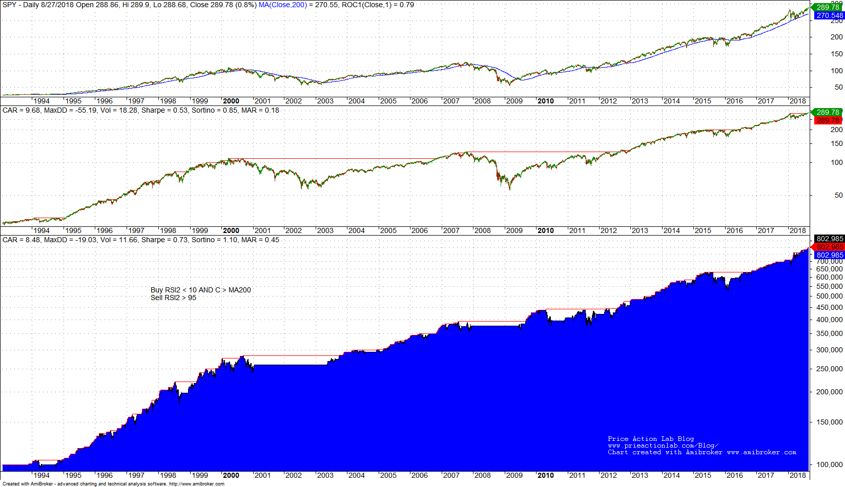
For example, one could use a (price > 200-day moving average) filter in an attempt to limit losses during bear markets while maintaining profits during bull markets. For the RSI2 strategy with OS = 10 and OB = 95, this is how the equity curve looks like for SPY since inception.
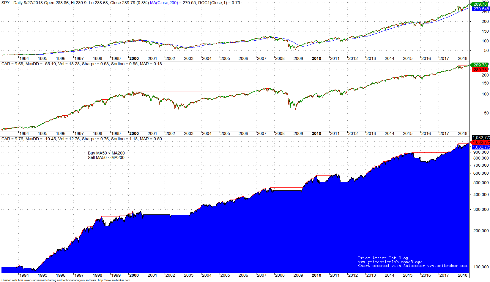
The maximum drawdown falls significantly and as a result MAR increases to 0.45. However, below is the performance of a long-only 50/200 cross strategy:
The moving average cross outperforms the RSI2 strategy with the bear market filter on both absolute and risk adjusted basis. Below is a comparison table.
| Parameter | RSI2+filter | 50/200 cross |
| CAGR | 8.48% | 9.76% |
| Max DD | -19.0% | -19.4% |
| Sharpe | 0.73 | 0.76 |
| MAR | 0.45 | 0.50 |
In other words, the trend is more important than the entry signal due to RSI. As it turns out then, the impact of the RSI2 signal is random.
Finally, some experienced developers use the RSI2, or variations thereof, for portfolio strategies, mainly long-only. In such cases the RSI2 may serve as a ranking mechanism but again its effectiveness depends on the value of the parameters and varies depending on market conditions.
If you found this article interesting, I invite you follow this blog via any of the methods below.
Subscribe via RSS or Email, or follow us on Twitter
If you have any questions or comments, happy to connect on Twitter: @mikeharrisNY
Charting and backtesting program: Amibroker
Technical and quantitative analysis of Dow-30 stocks and 30 popular ETFs is included in our Weekly Premium Report. Market signals from systematic strategies are offered in our premium Market Signals service.


